When twitter avatars recently went from square to circular, even though my old image had a circle in the centre, the cropping they picked meant it ended up looking even more ugly than before.
So now seemed like a good time to update it, and at the same time replace the old thndl logo with something fresher.
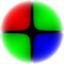
As usual, my go-to tool for this kind of thing is not to sketch in a drawing app, but instead to write a little shader program. You can already see the result in the top left corner of your page, but this is the short story of how it was constructed.
Making a picture using (mostly) code
I used shadertoy for the development. Here is the GLSL code I ended up with:
void mainImage( out vec4 fragColor, in vec2 fragCoord )
{
    vec2 uv = (fragCoord.xy - iResolution.xy*.5)/(iResolution.y*.5);
    float r = length(uv);
    float mask = 1.0-pow(r,10.0);
    vec2 c = mod(uv,2.0)-1.0;
    float f = length(pow(abs(c.xy),vec2(3.9)));
    float e = (1.0-smoothstep(0.84,0.85,f));
    vec2 q = sign(uv);
    vec3 col = vec3(1.0-step(q.y-q.x,0.0),step(-q.x*q.y,0.0),1.0-step(q.x-q.y,0.0));
    vec3 ec = mix(col,0.5*col,f);
    ec = mix(vec3(.0),ec,e);
    ec = mix(vec3(1.0),ec,mask);
    fragColor = vec4(ec*mask,mask);
}
Here is the resulting logo image rendered a bit larger:
While shadertoy is a great learning environment & community, it actually isn’t ideal for this kind of use case, where the final asset is not just something meant to be viewed through shadertoy.
One particular issue I hit was that even though you can easily save out a frame as a PNG (just right-click on the shader render view), shadertoy doesn’t currently (in Aug'17) support alpha channels, so you can’t make non-rectangular or masked images.
To work around that I actually had to save two image files - first the RGB image, and then a second grayscale mask image to convert to an alpha channel and combine using GIMP.
It’s a shame, because shadertoys do actually emit an RGBA value, it’s just that the A is currently thrown away.
Breaking it down
Now you’ve seen the code, and the finished article, let’s break it down line-by-line to understand exactly how that code turns into the final results.
For the visualisation, grayscale is used for float values, red-green for vec2s, and
RGB for vec3s. In each case we scale the parameter to fit into the 0-1 range.
(Note: the next sections are all rendered with WebGL, so if your browser doesn’t support that I’m afraid you won’t see any images. But since it’s already 2017, I assume most browsers can handle basic WebGLv1 well by now.)
Establishing Coordinate Space
The first line is:
vec2 uv = (fragCoord.xy - iResolution.xy*.5)/(iResolution.y*.5);
This establishes an x-y coordinate space with the same scale in both axes. This scaling is needed so that we can create a circle regardless of the canvas aspect ratio.
The Circular Mask
Next we’re going to create a single channel circular mask with the following two lines, visualised in the two images.
float r = length(uv);
float mask = 1.0-pow(r,10.0);
Squircles
Next we want to create a grid of squares, to suggest camera sensor pixels. These are based on squircles, and are defined with the following three lines, visualised in 3 images.
vec2 c = mod(uv,2.0)-1.0;
float f = length(pow(abs(c.xy),vec2(3.9)));
float e = (1.0-smoothstep(0.84,0.85,f));
The Bayer Matrix
Now we have the shape for the sensors, but we need to find a way to create the typical colour layout of a bayer matrix image sensor. Those have two greens for each red and blue.
Again for this, we need 3 lines of code. The middle one is a little complex, as it selects the correct combination of red, green or blue depending on the signs of x and y in that quadrant. The last line also mixes in the squircle to create a highlight.
vec2 q = sign(uv);
vec3 col = vec3(1.0-step(q.y-q.x,0.0),step(-q.x*q.y,0.0),1.0-step(q.x-q.y,0.0));
vec3 ec = mix(col,0.5*col,f);
Putting it all together
Finally we take the three streams, and put it all together with the last 3 lines. The final output line uses the circular mask also to create the alpha channel, so that the outline of the circle blends smoothly with the background.
ec = mix(vec3(.0),ec,e);
ec = mix(vec3(1.0),ec,mask);
fragColor = vec4(ec*mask,mask);
And we are done.
Why bother with all this?
Lots of reasons!
In this page I used WebGL to render the intermediate stages of the image. With the same rendering code, it only took a few minutes to arrange snippets of the same source code inline in the page like this - I didn’t need to spend time in my image editor preparing multiple PNGs and adding those to the assets.
Those code fragments are tiny and compressible compared to the equivalent PNGs, saving space and download time.
I have full access to all the parameters of the model, for instance the sharpness of edges, and those can be easily tweaked for variants or even animations.
And of course performance - shaders run entirely on your GPU, so your CPU and memory bus is kept quite idle when drawing these.
At least in theory. In practical use on the web, there are still some limitations preventing these benefits in some cases. While developing the WebGL code for this page, I noticed that on some platforms (e.g. Chrome for Android) there is a strict limit on the number of simultaneous WebGL contexts. So I had to modify the javascript code to render and then convert the result to an Image element. While this still makes editing easier, and cuts download time, it does increase local CPU processing and memory consumption.
Maybe in the future WebGL will get better at these kind of cases so that high performance shaders can be easily used throughout a normal page for all the graphics…
I made a slight improvement on the technique described above. Instead of an Image element, it now saves the data as an array using WebGL’s readPixels, and then creates a new canvas with a 2D context to put that back on screen. This should be slightly faster that the Image element approach.