Now we have a function which can give us a random-ish looking number between 0-1 for every pixel we render with a shader.
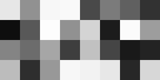
By using floor as we did earlier with continuous numbers, we can now have a random number for each different region of the image.
float rand(vec2 p) {
    p+=.2127+p.x*.3713*p.y;
    vec2 r=4.789*sin(489.123*(p));
    return fract(r.x*r.y);
}
f=vec4(rand(floor(vec2(4.,2.)*c.xy)))
We've put our random number code into a reusable function called rand(), with a couple of improvements compared to the original version.
First we skew the coordinates to avoid obvious symmetry - that also helps give us less aliasing patterns. That then allows the multiplier to be reduced to give us more precision when zooming out.
By scaling our coordinates and applying floor before calling the rand function, we can control how many regions we want.
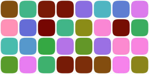
Putting together many techniques from earlier articles gives us, as an example, 32 random hued squircles.
float rand(vec2 p) {
    p+=.2127+p.x*.3713*p.y;
    vec2 r=4.789*sin(489.123*(p));
    return fract(r.x*r.y);
}

vec3 h2r(vec3 hsv) {
    vec3 t=clamp(abs(mod(hsv.r*6.+ vec3(0.,2.,4.),6.)-3.)-1.,0.,1.);
    return hsv.b*hsv.g*t+hsv.b-hsv.b*hsv.r;
}

vec2 p=c.xy*vec2(4.,2.);
float s=smoothstep(.1,.2,1.-length(pow(2.*fract(p)-1.,vec2(2.))));
vec3 t=h2r(vec3(rand(floor(p)),.75,.6));
f=vec4(t,s)
Ok, so that's one basic use for randomness to raise the interest level of shaders.
The next thing we need to make is, a little perversely, smoothed noise.
You see, the problem with the noise we've made so far is that it's "white noise" with about the same amount of power at all frequencies.
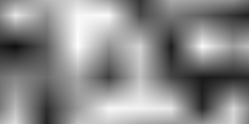
By smoothing - filtering - it, we can create a different spectrum of noise. The simplest way to do this is to use the floor to calculate the 4 random values around each point, and then blend those values based on how far the point is from each one.
Something like this:
float rand(vec2 p) {
    p+=.2127+p.x*.3713*p.y;
    vec2 r=4.789*sin(489.123*(p));
    return fract(r.x*r.y);
}
float sn(vec2 p) {
    vec2 i=floor(p-.5);
    vec2 f=fract(p-.5);
    float rt=mix(rand(i),rand(i+vec2(1.,0.)),f.x);
    float rb=mix(rand(i+vec2(0.,1.)),rand(i+vec2(1.,1.)),f.x);
    return mix(rt,rb,f.y);
}
f=vec4(vec3(sn(vec2(4.,2.)*c.xy)),1.)
That was blending with 3 normal mix statements - bilinear smoothing. It would look much better with one line added to modify the fract and make a non-linear blend.
The equivalent of a smoothstep would be f=f*f*(3.0-2.0*f). But an even better alternative (which is smooth also at higher derivatives) comes via Inigo Quilez: f = f*f*f*(f*(f*6.0-15.0)+10.0)

float rand(vec2 p) {
    p+=.2127+p.x*.3713*p.y;
    vec2 r=4.789*sin(489.123*(p));
    return fract(r.x*r.y);
}
float sn(vec2 p) {
    vec2 i=floor(p-.5);
    vec2 f=fract(p-.5);
    f = f*f*f*(f*(f*6.0-15.0)+10.0);
    float rt=mix(rand(i),rand(i+vec2(1.,0.)),f.x);
    float rb=mix(rand(i+vec2(0.,1.)),rand(i+vec2(1.,1.)),f.x);
    return mix(rt,rb,f.y);
}
f=vec4(vec3(sn(vec2(4.,2.)*c.xy)),1.)
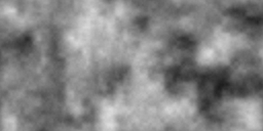
Finally, we can create a controlled spectrum of noise by using this function to generate smooth noise at different frequency octaves.
For example, we can double the frequency each time, and then add them all together with different strengths. The most common approach is to halve the strength of each octave higher. Like this:
float rand(vec2 p) {
    p+=.2127+p.x*.3713*p.y;
    vec2 r=4.789*sin(489.123*(p));
    return fract(r.x*r.y);
}
float sn(vec2 p){
    vec2 i=floor(p-.5);
    vec2 f=fract(p-.5);
    f = f*f*f*(f*(f*6.0-15.0)+10.0);
    float rt=mix(rand(i),rand(i+vec2(1.,0.)),f.x);
    float rb=mix(rand(i+vec2(0.,1.)),rand(i+vec2(1.,1.)),f.x);
    return mix(rt,rb,f.y);
}
vec2 p=c.xy*vec2(4.,2.);
f=vec4(vec3(
    .5*sn(p)
    +.25*sn(2.*p)
    +.125*sn(4.*p)
    +.0625*sn(8.*p)
    +.03125*sn(16.*p)+
    .015*sn(32.*p)),1.)
This kind of cloudy pattern is usually called Fractional Brownian Motion (FBM). As you can see, it's very expensive to calculate - in our case needing no less than 48 sin() calls for each pixel - ouch!
But it makes an incredibly useful and reusable building block for modulating and colouring other simpler functions to give shader images a more natural or organic feeling.
Here's one example to end with, an instant world map.
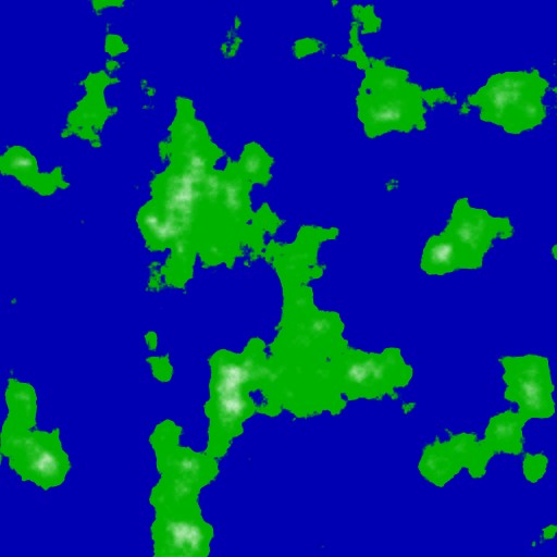
float rand(vec2 p) {
    p+=.2127+p.x+.3713*p.y;
    vec2 r=4.789*sin(789.123*(p));
    return fract(r.x*r.y);
}
float sn(vec2 p) {
    vec2 i=floor(p-.5);
    vec2 f=fract(p-.5);
    f = f*f*f*(f*(f*6.0-15.0)+10.0);
    float rt=mix(rand(i),rand(i+vec2(1.,0.)),f.x);
    float rb=mix(rand(i+vec2(0.,1.)),rand(i+vec2(1.,1.)),f.x);
    return mix(rt,rb,f.y);
}
float bm(vec2 p) {
    return .5*sn(p)
    +.25*sn(2.*p)
    +.125*sn(4.*p)
    +.0625*sn(8.*p)
    +.03125*sn(16.*p)+
    .0156*sn(32.*p);
 }
float h=bm(c.xy*4.);
f=vec4(mix(mix(vec4(0.,0.,.7,1.),vec4(0.,.7,0.,1.),smoothstep(.6,.63,h)),vec4(1.),smoothstep(.7,.95,h)))